The Extragalactic Distance Scale
Distances to galaxies and AGNs are important, but direct means of measuring
distances may be difficult and very time-consuming. Hence the mere
possibility of something like the Hubble flow cz = H0 D
would be a real
boon, since we could then estimate distance (to within errors caused by
peculiar motion) from a single straightforward measurement. The idea is then
that for "large enough" D, the Hubble velocity will overwhelm any
peculiar motions and we will see a smooth, purely radial flow.
Finding the value of H0 has been an important part of galaxy research
from its inception, with the recent additional possibility of mapping
systematic departures from a smooth Hubble flow. The procedure usually
follows a distance ladder, in which objects of well-known properties
are used to calibrate larger/brighter kinds of objects which can in turn be
used to calibrate other indicators that may be seen to greater distances,
until finally we have indicators that are useful into the realm of
allegedly pure cosmological motion. A distance indicator must have the
following attributes:
It must have known properties (size, luminosity)
that do not depend in an "invisible" way on
distance or environment. Recall that distance measures appropriate for size
and luminosity may differ over cosmologically long lines of sight.
Any variation between such standard candles must have some
observable effect (i.e. period-luminosity law for Cepheids, or
decline-luminosity correlation for SN Ia).
We must be able to calibrate these indicators, either directly
or via other distance indicators.
Their scatter must be small or well known, to avoid Malmquist bias.
Much of the debate over the distance scale arises from the large distances
that we need to cover to be sure we are beyond the range of peculiar
velocities such as Virgocentric flow. Eventually, we find that only global
galaxy properties and their correlations are usable. In the ladder
of distance indicators, propagation of errors becomes dominant. See
Rowan-Robinson, The Cosmological Distance Ladder (Cambridge 1987),
for a full discussion. Modern methods are described in Galaxy
Distances and Deviations from Universal Expansion, ed. B. Madore and R.B.
Tully (NATO ASI 180). We will consider the methods in the traditionql
distance ladder in turn.
Trigonometric parallax. This is useful out to a few hundred pc
for individual stars if we have milliarcsecond precision, which
Hipparcos delivered for tens of thousands of stars. This is the only
(almost) completely
foolproof technique for distances, since we know the size of the Earth's
orbit well. Statistical applications can be applied to whole groups of
stars, using (for example) the solar motion through the galactic disk to
generate secular parallax. These still sample only a tiny region of
the galaxy, and in particular do not reach to either very luminous stars or
Cepheid variables (though Hipparcos delivered statistically useful
parallaxes for some Cepheids).
Cluster convergent points. For nearby clusters of
appreciable angular extent (like the Hyades)
perspective makes the proper motions of individual stars not parallel, but
directed toward a point in the sky parallel
to the cluster's mean motion relative to the Sun. This gives the angle
between our line of sight and the cluster's motion, and thus what fraction
of the cluster's space motion is seen as proper motion and what as radial
velocity. Measuring the average radial velocity then allows a distance
determination, as the distance for which the radial velocity and proper
motion are consistent with the angle between line-of-sight and space
motion. This lets us calibrate absolute magnitudes for all the cluster
members - including upper main-sequence and red giant stars.
The classic example
is the Hyades cluster, seen here using Hipparcos proper
motions from Perryman et al. (1998 A&A 331, 81):
Main-sequence fitting. For even more distant star clusters (that
might contain OB stars or Cepheids, for example) we estimate distances
by assuming that main-sequence stars of identical spectral type have the
same absolute magnitude. This amounts to, for example, shifting the
main-sequence location of a cluster until it coincides with that of some
reference cluster like the Hyades. The reddening must be
reasonably well determined to make this work. This can be done for systems
as distant as the Magellanic clouds, which is the easiest place to
calibrate Cepheids. For this purpose, each Magellanic Cloud can be thought
of as a giant cluster.
Cepheid variables. These are supergiants in the instability
strip on the H-R diagram, undergoing regular pulsations that are expressed
by luminosity and temperature variations. Their high optical luminosity
makes them easy to pick out (though, being rather massive stars, they
don't occur in elliptical galaxies). Recent data give a period-luminosity
relation of the form
<MV> = -3.53 log P + 2.13 (<B0> -
<V0>) +
φ
where φ
~ -2.25 is a zero point. P is in days here, and the
brackets denote averaging over a cycle of the light curve. The relations for
the SMC and LMC are shown by Mathewson, Ford and Visvanathan 1986 (ApJ 301, 664)
as follows, from their Fig. 3 (courtesy of the AAS):
To use Cepheids effectively, one must deal with the following points:
P and <V> must be adequately defined - there must be enough
measurements of suitable spacing. Working out the minimum acceptable
number of observations, and their spacing, to avoid missing large numbers
of Cepheids, is an interesting HST scheduling problem, showing another
less-obvious advantage of being beyond the atmosphere.
Possible shifts of the P-L relation with metallicity. This seems
not to be as big an issue as once thought; there is some evidence that
the metallicity effects act mostly parallel to the instability strip
rather than shifting it mainly in termperature (or period).
Reddening corrections. To some extent, this may be obviated by
near-IR photometry of Cepheids once they have been selected from optical
images (for example, Welch et al. 1986 (ApJ 305, 583). Not least, this
affects our absolute calibration by producing difficulties in our own
galaxy - Cepheids are rare and relatively young, which means we see them
through large path lengths of galactic dust.
Crowding from surrounding stars altering their observed
magnitudes (going to the IR may help here as well as the obvious
tack of HST observations). Recent simulations have reached divergent
conclusions as to how important this effect will be on the HST Key
Project results. Sigh.
Cepheids have been measured from the ground throughout the Local Group
(which Hubble could do - the astronomer, not the telescope), and can be detected
in the M81 and Sculptor groups, and more recently in M101 at a distance of
7 Mpc (Cook, Aaronson, and Illingworth 1986 ApJLett 301, L45), and even
an amazing detection of a couple in the late-type Virgo spiral NGC 4751, when
the seeing and stellar crowding all worked together
(Pierce et al. 1994 BAAS 26, 1411). Note that
it is traditional to quote the distance modulus m-M = 5 log D - 5
rather than the distance itself
in many publications on the distance scale - for example, the DM of the LMC is
close to 18.5. To date, the HST key project
on the distance scale has reported detections of Cepheids to 25 Mpc,
and it can in principle go well beyond Virgo. A real shame there aren't
any spirals which can be shown to live in the Coma core. The best-known
report of this work was for NGC 4321=M100 in Virgo by Ferrarese et al
(1996 ApJ 464, 568), see also Freedman et al 1994 (Nature 371, 757).
The project, using Cepheids to calibrate secondary distance
indicators through common galaxy and group membership, was described by
Kennicutt, Mould, and Freedman 1995 (AJ 110, 1476). Some of their
Cepheid light curves are shown below -- for M100 alone, they already
detect more Cepheids than are known in the LMC, so the LMC calibration
becomes a weak link. The project has gotten all its data, and a recent
summary (Mould et al. 2000 ApJ 529, 7867) gives a grand average value of
H0= 71 ± 6 km/s Mpc as based on HST Cepheid distances
to 25 galaxies, in ridiculously close agreement with results of
fitting the WMAP power spectrum of CMB fluctuation.
This plot colects the Key Project Cepheid distances. Note the
large peculiar motions within Virgo; the one galaxy lying right on the
mean line at that distance is NGC 7331, almost opposite Virgo in the sky.
RR Lyrae stars. These are lower-luminosity stars, where the
instability strip crosses the horizontal branch. They may appear on cluster
H-R diagrams by omission in the "RR Lyrae gap", since variables are
usually not plotted. The absolute magnitude of all RR Lyrae variables seems
to be nearly constant at
<MV = 0.75 ± 0.1.
There may be some poorly-determined metallicity dependence. No period
determination is needed here, just the determination that a star is of this
type (which means you get the period anyway). Problems are: RR Lyraes are
intrinsically about 2 magnitudes fainter than Cepheids, and similarly
difficult to calibrate; only a couple are close enough for a parallax
measurement with
Hipparcos, so statistical parallaxes are still important.
Automated image detection has proven fruitful in finding these stars
throughout the Local Group, even before HST. Saha and Hoessel (1990, AJ 99, 97)
report
finding 151 in the small elliptical NGC 185, as seen
in their Fig. 5 courtesy of the AAS:
Most luminous (blue/red) stars. There is an empirical relation
between a galaxy's absolute magnitude and that of the brightest individual
stars - this amounts to assuming a constant form for the upper end of the
luminosity function and letting statistics operate. Conveniently, these are
the first stars to be resolved. Possible problems: confusion with compact
clusters (as in 30 Doradus), unknown variation with galaxy type.
All of the stellar indicators listed above for other galaxies are easiest to
use in systems with substantial population I components, and in rather open
galaxies so that crowding is reduced. One therefore tries to deal with a
galaxy's outer regions, and rather late-type galaxies (see the Sandage and
Bedke atlas for illustrations of resolution into stars for such galaxies,
which was the point of their producing this volume).
There are also several temporary or indirect stellar distance indicators:
Novae. There is a relation between absolute magnitude and
fading rate for novae, as best we can tell from the Local Group. They can
easily be picked out as transient
Hα
sources, and two seem to have
been detected in this way as far away as M87 (Pritchet and van den Bergh 1987
ApJLett 288, L41); as well, data series sufficient to find Cepheids
may find them as continuum sources. Ciardullo et al. (1990 ApJ 356, 472)
discuss 11 well-observed
novae in M31. The relation between fading rate and absolute B magnitude is
only partially followed by
Hα,
so that a combination of
Hα
discovery, continuum observations near maximum, and
Hα
observations
to faint levels seems the most effective approach. Faint continuum
measurements are impossible because the nova blends into the overall
stellar background. This technique may be used for population II systems.
Planetary nebulae. These can also trace the population II
components, since they can be produced by old stars. Their usefulness as a
distance indicator relies on the fact that their luminosity function
appears to be invariant, and is easily understood from stellar evolution
(Jacoby 1989 ApJ 339, 39). Large numbers of planetaries can be detected
in nearby galaxies by using narrow-band images around the [O III]
λ5007
line, which is extremely strong in planetaries but not most H II
regions. Sufficient planetaries have been detected for estimates of the
distance to Virgo (Jacoby et al. 1990, ApJ 356, 332). The fitting technique
for an incomplete luminosity function is illustrated by Fig. 3 of
Ciardullo et al. 1989 (ApJ 339, 53) for M31 (courtesy the AAS):
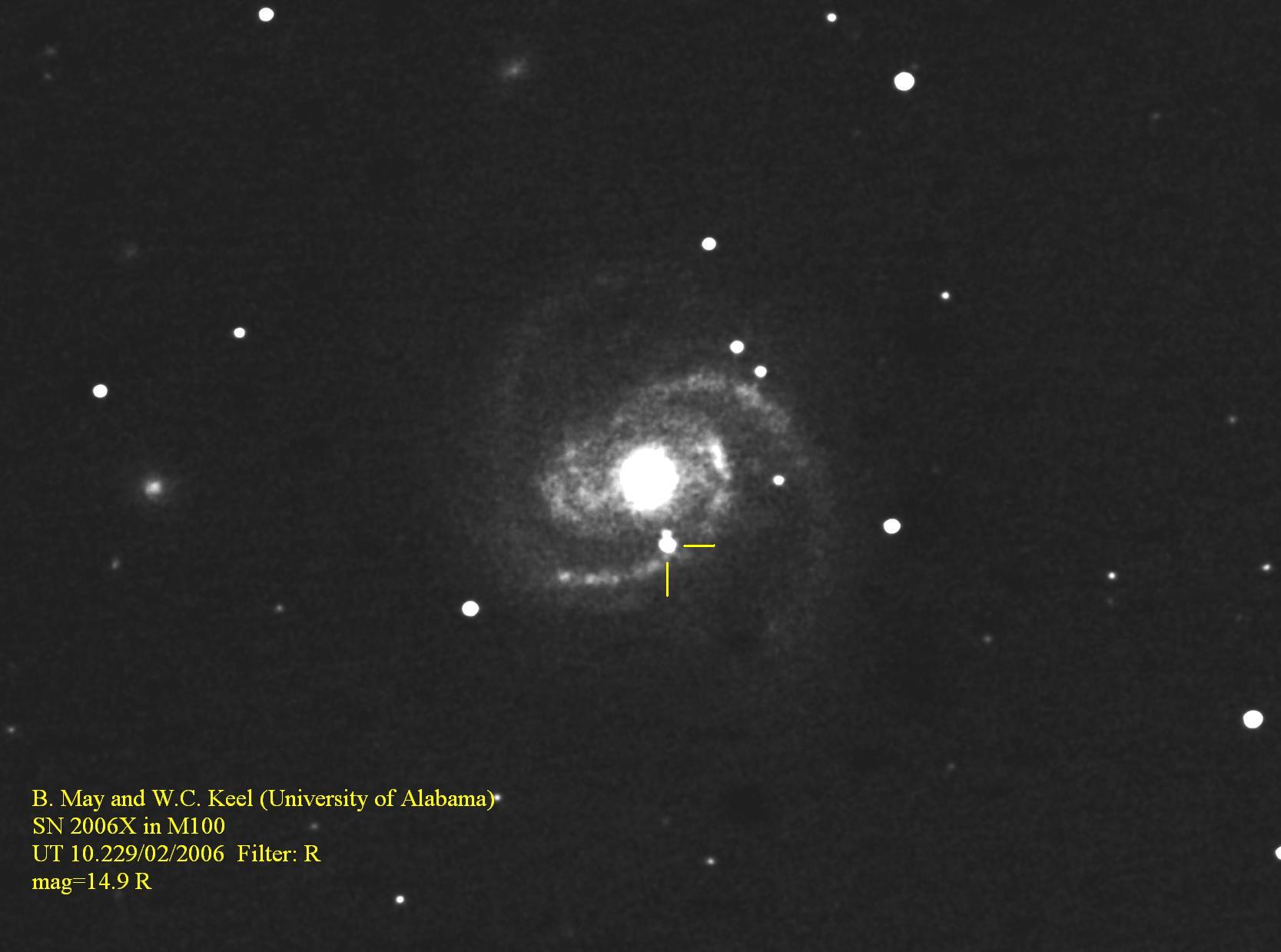
Supernovae. Type I (population II) supernovae can be
recognized (and divided into subgroups a,b, and maybe c) based on their
spectra and light curves. Available evidence is consistent with peak
luminosity being roughly fixed for at at least type Ia
(but watch out, new understanding of
subluminous ones like 1987A may change this). Supernovae can be seen a
long way off (like z=1.7 if you're looking hard), so they would make
wonderful distance indicators if (1) we really know this peak luminosity,
(2) it really is constant, and (3) we can account for dust obscuration
(hello IR). The peak brightness is given by supernova models, but SN in
galaxies nearby
enough for checking are rare. For cosmologically
distant SN the rate of decay is stretched by the dilation factor (1+z).
These are the objects which first provided strong evidence for
an acceleration of the Hubble expansion (perhaps to be identified with
Einstein's cosmological constant).
A direct measure of distance for expanding or pulsating objects is in
principle possible via the Baade-Wesselink method. One measures the change
in bolometric luminosity and the integral (change in relative)
radial velocity over this time.
Then, applying either a blackbody approximation or a more realistic
spectrum, the angular size difference between two epochs is derived, which
gives a distance by requiring it to be consistent with the radius change
from radial velocities. Problems center around just how the observed
velocity is weighted across the photosphere and whether the opacity
structure changes between epochs.
 Surface-brightness fluctuations. Well
before a galaxy is truly
resolved into even its brightest stars, the image will be mottled by statistical
fluctuations; for example, if the surface brightness is such that there are
100 red giants per seeing disk, one expects 10% Poisson fluctuations.
These may be distinguished from photon noise because these fluctuations
have the same spatial power spectrum as the seeing disk (or more generally
the system response, i.e. PSF), not white noise
(Tonry and
Schneider 1988 AJ 96, 807). As a sample, this image
shows M32 HST data resampled
as if seen at progressively greater distances (each step increasing
by a factor 2). The technique is surprisingly powerful as long
as one can compare galaxies with similar stellar populations - basically
one must assume a characteristic (well-defined) mean luminosity for stars.
The method has already been extended to Virgo, giving excellent agreement
with planetary-nebula determinations and first hints as to which galaxies
are on the near and far sides (Tonry et al. 1989 ApJ 346, L57).
Surface-brightness fluctuations. Well
before a galaxy is truly
resolved into even its brightest stars, the image will be mottled by statistical
fluctuations; for example, if the surface brightness is such that there are
100 red giants per seeing disk, one expects 10% Poisson fluctuations.
These may be distinguished from photon noise because these fluctuations
have the same spatial power spectrum as the seeing disk (or more generally
the system response, i.e. PSF), not white noise
(Tonry and
Schneider 1988 AJ 96, 807). As a sample, this image
shows M32 HST data resampled
as if seen at progressively greater distances (each step increasing
by a factor 2). The technique is surprisingly powerful as long
as one can compare galaxies with similar stellar populations - basically
one must assume a characteristic (well-defined) mean luminosity for stars.
The method has already been extended to Virgo, giving excellent agreement
with planetary-nebula determinations and first hints as to which galaxies
are on the near and far sides (Tonry et al. 1989 ApJ 346, L57).
H II regions. By necessity these require active star
formation and OB stars. They are luminous and measurable to very large
distances. The first approach (Sandage and Tammann 1974 ApJ 190, 525) was
to assume that the diameter of the brightest H II regions is related
to galaxy absolute magnitude. However, Kennicutt 1979 (ApJ 228, 704) showed
that seeing effects compromise visual and isophotal diameters so strongly
that this cannot work as a distance indicator. More recent work has focussed
on emission-line luminosities, assuming in essence that the more star
formation, the brighter the galaxy, and statistically the brighter the
biggest few H II regions are. This might be considered a variant on the
brightest blue stars method.
The emission-line widths have also been considered, with a claim by
Terlevich and Melnick (1981 MNRAS 195, 839)
that an
L - σ4
relation holds for supergiant
H II regions; that is that they are bound by a gravitational mass
propertional to (ionizing-UV) starlight intensity.
This would be useful in the same way
as the Tully-Fisher relation or the analogous relation for elliptical
galaxies. However, further work (Gallagher and Hunter 1983 ApJ 274, 141;
Roy et al. 1986 ApJ 300, 624) has clouded the picture; for more extended
samples, the correlation is much less striking, and the gas motions are
largely supersonic, driven by stellar winds and SN rather than being
gravitationally produced.
Galaxy structures. We may consider identifiable structure
within galaxies as distance indicators, if they have constant or
calibratable sizes. Candidates have included:
Inner rings - see Buta and de Vaucouleurs 1983 ApJ 266,1 and
references therein. These are statistically useful, but not competitive with
other methods - not least because most galaxies don't have these
structures.
Widths of spiral arms (Block), using an empirical relation
between linear width of arms and galaxy luminosity. The possibility of
distance determinations arises because the brightness-distance and
angular size-distance relations have different slope.
Globular-cluster luminosity functions - these work much like the
planetary-nebula luminosity function technique. Globulars have been
observed in detail in Virgo (i.e. Harris and van den Bergh 1981 AJ 86, 1627)
and as far away as the Coma cluster
(Harris 1987 ApJLett 315, L29, Baum et al. 1995 AJ 110, 2537).
Available data are at least consistent with
the globular-cluster luminosity function being universal for various galaxy
types, though the number of clusters varies widely.
Central velocity dispersions of elliptical galaxies - the
Faber-Jackson relation (1976 ApJ 204, 668) otherwise known as the
L - σ4
relation (a manifestation of the fundamental plane, as we've
discussed). As shown in their Fig. 16, the correlation is
reasonable; a rough theoretical argument has been applied, assuming the L
measures total mass in some scaled way.
A refinement, including a second parameter
related to surface brightness, has been used by the Seven Samurai to compile a
large set of
redshift-independent distances for mapping the local velocity field
(Dressler et al. 1987 ApJ 313, 42; data in Faber et al. 1989 ApJSuppl 69,
763).
Global galaxy properties: These must be used for more and more
distant systems, requiring extensive calibration from the techniques above.
Specific indicators include:
"Sosies": from the French for lookalikes. The idea here is
to find galaxies that look as much like our own or a very nearby one
as possible, assuming then
that lookalikes have the same size and luminosity. This has been applied by
Paturel 1984 (ApJ 282, 382) and Bottinelli et al. (1985, ApJSuppl 59, 293).
The morphological type of the Milky Way was taken as SAB(rs)bc, as
classified by de Vaucouleurs. This is very Copernican in its assumption of
mediocrity on our part.
Luminosity classes. As discussed on p. 12, there is a
general correlation between arm structure and absolute magnitude for
spirals, especially Sc systems. The distribution, of course, turns out to
be broader than once thought (see the Sandage and Bedke atlas), so this is
not such a good primary indicator.
H I linewidth: Tully and Fisher (1977 A&A 54, 661)
found an excellent
correlation between the peak separation in an H I profile (corrected to
zero inclination) and absolute magnitude for spirals. An important
improvement used by Aaronson, Huchra, and Mould 1980 (ApJ 229, 1) was the
use of near-IR H magnitudes to reduce effects of dust and recent star
formation; this is perhaps the most widely useful and accurate distance
indicator for surveys. They calibrate the slope of the T-F relation for the
Virgo cluster and nearby groups, and set the zero point from M31 whose
distance is independently known. Their results led to the complex
Virgo-infall model that is now seen to complicate local distance
measurements. There remains some dispute over whether the zero point of the
T-F relation depends on Hubble type. More recent work has extended such
survey data around the sky, and shown evidence for larger-scale
motions superimposed on the Hubble flow (such as the search
for the "Great Attractor" in the southern sky).
Brightest cluster members: for rich clusters, one expects
the brightest galaxies to have almost the same absolute magnitude, simply
because the galaxy LF drops so steeply at the bright end that one would
need huge numbers of galaxies to change this by much. The very brightest
tend to a fixed luminosity (perhaps some special process is at work in
their formation). These can be seen to extreme distances (like z=2.5),
and are often used to search for evolutionary effects. One cannot
simultaneously use galaxy fluxes to
look for luminosity evolution and distance without
other information!
Corrections to observed magnitudes must be applied for (1) measuring
aperture size (2) passband redshifting, the so-called K-correction (3)
the redshifting of both photon energy and arrival rate, and (4) any assumed
evolution - at least passive evolution of the stellar population must be
taking place.
"Exotic" Distance Indicators
All of the above methods rely on a straightforward application of the
inverse-square law or the angular diameter-distance relation. There is also
a range of techniques that use more involved or indirect combinations of
observables. Some examples are:
The Hubble time: for simple big-bang models, ages of objects
(stars, radioactive nuclei) set bounds on H0. The age of
the universe is
of order the Hubble time
τH
=1/H0, to within a factor of order
unity depending on the deceleration history of the expansion. For
H0=50 km/s Mpc,
τH= 2
x1010 years; for 100 km/s Mpc, 1010 years.
This must be greater than the age determined from geological and
stellar-evolutionary timescales, nuclear isotopic clocks like
235U/238U, and consistent with the dynamical
status of galaxies
and clusters. The small amount of evolution observed in elliptical galaxies
to about z=1 favors smaller H0 in simple models
(Hamilton 1985 ApJ
297, 371). One should beware subtly circular arguments - globular-cluster
ages were beautifully consistent with H0=50 but had been
calculated by
people who know the answer they expected to get and tuned a few parametere
accordingly. There was, for several years, a widely-publicized
discrepancy between
τH
from HST Cepheid results and globular-cluster
ages, but recent calculations of effects of mixing on stellar evolution
and the Hipparcos distance revisions to Cepheids
both go in the direction of reducing the problem.
Gravitational lenses: we need to know the lens mass (for
example through the cluster velocity dispersion) and the time delay between
images (say from QSO variability). Then we can derive the lens proper
distance. The differential time delay may be the hardest part here,
especially in the presence of microlensing.
Light echoes: this has given an independent distance to the
LMC, by using the time of illumination of a circumstellar ring (seen from
IUE, Panagia et al. 1991 ApJL 380, L23) to give an absolute front-back size,
and the angular size of the ring (from HST) for a transverse measurement.
This example
was done by, for example, Gould (1995 ApJ 452, 189).
A similar approach can also be used (with polarization
to tell where the ring is) for distant supernovae (Sparks 1994 ApJ 433, 19).
Emission/absorption measures: here one uses the different
dependences of emission and absorption on density versus path length. An
example is the IGM in clusters seen in emission via X-rays and in
absorption (more precisely upward scattering)
against the microwave background (the Sunyaev-Zeldovich effect).
This works because on astrophysical grounds we expect the hot gas
to be smoothly distributed through the cluster potential; clumping
would make this more useful for probing
structure than distance.
So far, this isn't accurate enough for use as more than
a consistency argument because the absorption is very
weak, but in principle is free of many of the assumptions of other methods
(107 K gas should be very smoothly distributed).
This technique for detecting hot cluster atmospheres is almost
equally sensitive for all cluster redshifts z>0.5
because it's an area measure, so surveys are in progress to find high-redshift
clusters as S-Z spots.
Proper motions: a maser in a star-forming region should be
detectable with the VLBA all the way to Virgo. Its proper motion due to
the rotation of a typical spiral should be of order 3 microarcseconds per year,
which, it has been claimed, should be measurable in a decade or so. One then
determines the distance at which this matches the disk rotational velocity
at the appropriate radius. The most distant actual application so far
has been to masers in the nuclear disk of NGC 4258 (Herrnstein et al.
1999 Nature 400, 539).
Distance estimates
Distances to nearby galaxies are not in serious dispute, but the role of
peculiar velocity on these scales is. Some useful distances are (in Mpc)
| Object | Distance |
| LMC | 0.05 |
| M31 | 0.68 |
| M81 group | 3.2 |
| Sculptor group | 3-3.5 |
| M101 | 4-5 |
| Virgo core | 14-18 |
| Coma cluster | 100 |
This means that H(Virgo) is about 60 km/s Mpc, but is this value globally
applicable? Two major camps long existed: Sandage at 50 (the "long" distance
scale) and de Vaucouleurs at 100 (the "short" scale). Data occasionally drown
in invective on this issue. Doing a systematic
error treatment, Hanes 1981 (MNRAS) and Rowan-Robinson in his book found
that 80 km/s Mpc satisfies all the error bars and is what the IR T-F
relation gives at large distances. This is essentially
the Key Project global value as well, with the CMBR global
fitting giving a value of 71. Maybe the compromise value of 75 that
many people have used was actually more than fence-sitting.
Non-Hubble Motions
Aaronson, Huchra, and Mould found evidence for systematic departures from
the Hubble flow toward Virgo, so that the redshift-distance relation is
nonlinear, and in some places double or triple-valued.
A first indication of such disturbances was the study by Rubin and Ford
(1987 AJ 81, 719) of 96 Sc I galaxies, which showed an asymmetry on the sky
in redshift-magnitude space such that we were likely to be moving at about
500 km/s with respect to the centroid of these galaxies.
This eventually turned into an industry, with the 7 Samurai
announcing a "Great Attractor" off in Centaurus (l=299°,
b=-11°) that messes up the
velocity field out to about 3000 km/s (Lynden-Bell et al. 1987 ApJLett 313,
L37). We are approaching this mass at about 700 km/s; this is actually
consistent with the Rubin and Ford result if Virgo infall is included.
Lauer and Postman (1994 ApJ 425, 418) find yet a different motion relative to
119 Abell clusters at z < 0.05 - 561 ± 284 km/s toward
l=220 °, b= -28 °, yet a different direction and
certainly an unexpected magnitude.
A somewhat different motion is derived with respect to the microwave
background, which is the grandest average we can find - the final
COBE data set gives 368 km/s toward l=264.3, b=48.1
with independent analysis of the FIRAS and DMR instruments in good agreement
(Lineweaver et al.
1996 ApJ 470, 38). This has just been refined with WMAP to
l=263.8, b=48.2 (Bennett et al. ApJ submitted,
astro-ph/0302207).
At some point one wonders about the the scale on which the
cosmological principle is adequately realized. This means that the
Grail itself, H0,
must be
sought at even larger distances than thought before (to the extent that
it would be useful in itself if the Hubble flow is really lumpy,
though the tightness of the Hubble diagram for standard candles
suggests that it isn't all that bad).
There are also isolated instances of galaxies flagrantly violating the
Hubble flow. Perhaps the best is in the direction of NGC 1275. The main
galaxy has v=5000 km/s, and has something that looks like a late-type
spiral demonstrably in front of it but having v=8100 km/s.
Images from Keel 1983 (AJ 88, 1579) isolate the foreground and background
systems in
Hα:
while the foreground system is visible in absorption by dust in
this HST image:

This is
too fast to be just free fall into a cluster core - and if there are many
galaxies shooting around at 3000 km/s there should be huge scatter in the
Hubble diagram. Thus there can't be many of these, but how far would we
have gone wrong if we saw the spiral by itself?
« Dark matter in galaxies
| Groups and clusters of galaxies »
Course Home |
Bill Keel's Home Page |
Image Usage and Copyright Info |
UA Astronomy
keel@bildad.astr.ua.edu
Last changes: 10/2009 © 2000-9